Undisclosed Client Final Analysis
In this notebook we will be looking for relationships between disease stage, mouse sex and group. We begin by the necessary libraries.
# required libraries
library(psych)
library(dplyr)
library(ggplot2)
library(knitr)
library(pander)
panderOptions('knitr.auto.asis', FALSE)
After importing libraries we will import the data.
# read the csv data and split into test and control groups
data <- read.csv("FinalAnalysisClientDataset.csv", header=TRUE, stringsAsFactors=TRUE)
data$BMP_2 <- sapply(sapply(data$BMP_2, as.character), as.numeric) #had to convert this column to numerics
test <- subset(data, Category == "Test")
control <- subset(data, Category == "Control")
Lets write some descriptive statistics on BMP_1 and BMP_2 levels so we understand what our data looks like.
# small summary of basic stats using describe
kable(describe(data$BMP_1, skew=FALSE), caption = "Descrpitive Statistics on BMP_1 levels")| vars | n | mean | sd | min | max | range | se | |
|---|---|---|---|---|---|---|---|---|
| X1 | 1 | 36 | 80.84 | 24.93527 | 41.943 | 154.72 | 112.777 | 4.155879 |
kable(describe(data$BMP_2, skew=FALSE), caption = "Descriptive Statistics on BMP_2 levels")| vars | n | mean | sd | min | max | range | se | |
|---|---|---|---|---|---|---|---|---|
| X1 | 1 | 102 | 254.1349 | 165.2406 | 68.84 | 730.17 | 661.33 | 16.36126 |
#create a box plot to illustrate data
ggplot(data, aes(x=Category, y=BMP_1)) + geom_boxplot()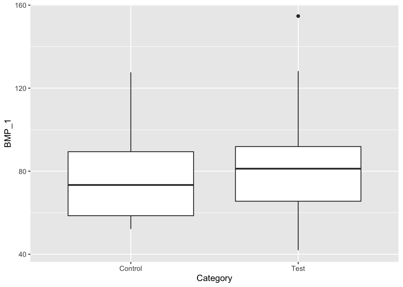
ggplot(data, aes(x=Category, y=BMP_2)) + geom_boxplot()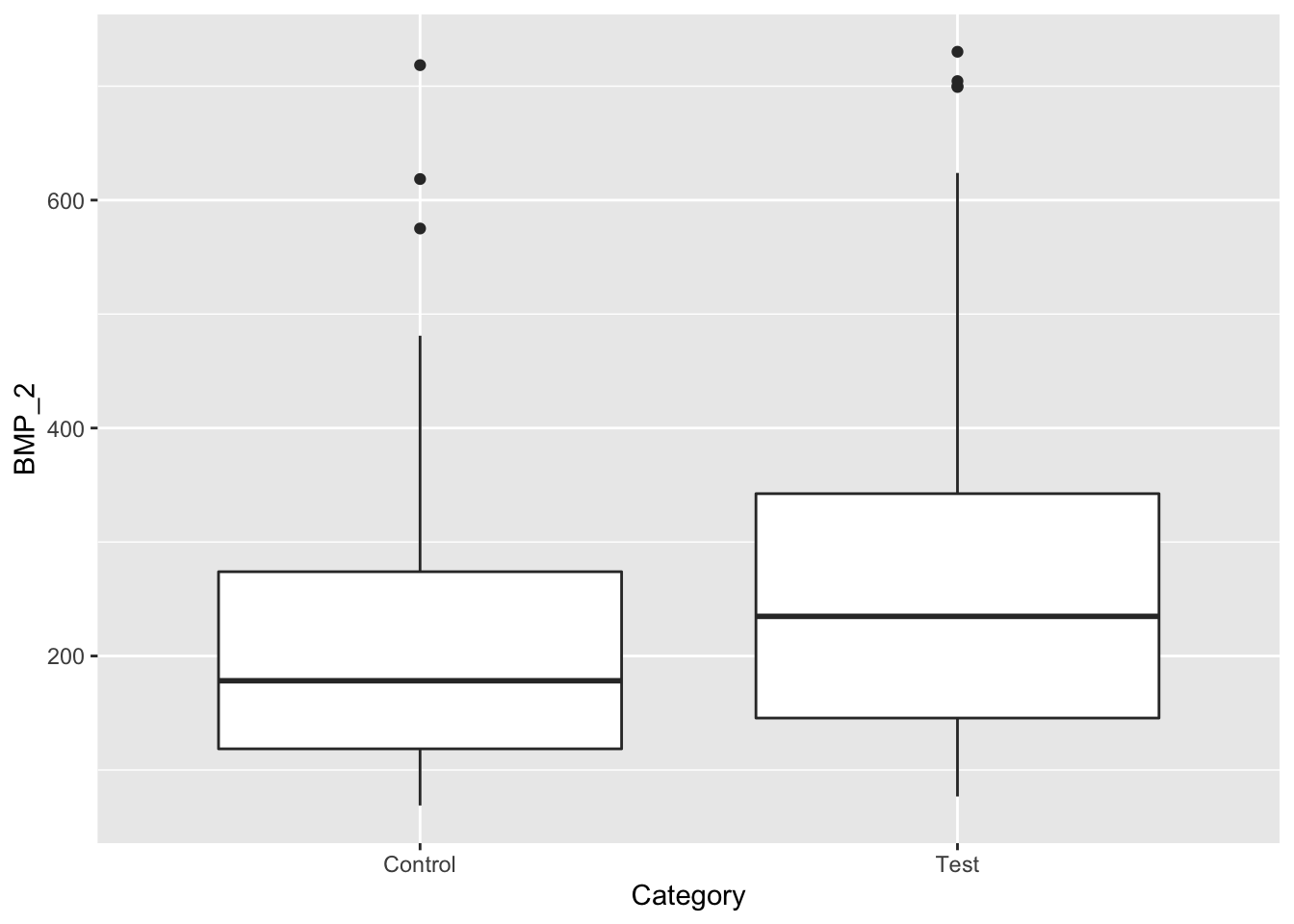
From this data we see that the mean BMP_2 and BMP_1 in the test groups are higher than their respective control groups. However, there is a lot of overlap based on these box-whisker plots. Lets try to further investigate this issue by looking at box-whisker plots for each subgroup. Mice can be grouped by disease stage, and gender, as illustrated in Table 3.
| Independent Factor | Levels | Level Names |
|---|---|---|
| Category | 2 | Test, Control |
| Age Group | 5 | Pre-symptomatic, Early Stage, Intermediate Stage, Late Stage, End Stage |
| Sex | 2 | Male, Female |
# Source https://r-graph-gallery.com/265-grouped-boxplot-with-ggplot2.html
# For BMP_2 we generate a grouped boxed plot for each disease stage, and participant sex
ggplot(data, aes(x=Age_group, y=BMP_2, fill=Category)) +
geom_boxplot() +
facet_wrap(~Age_group, scale="free")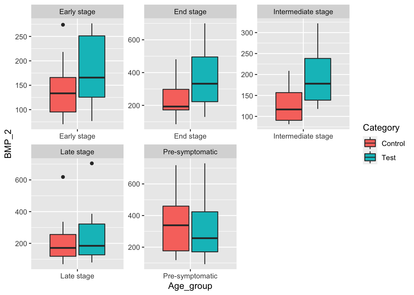 When creating box-whisker plots for BMP_2 levels when mice are grouped only by disease stage we see that the mean BMP_2 level is higher in the test group except for the Pre-symptomatic group. Lets see how BMP_1 levels compare.
# For BMP_1 we generate a grouped boxed plot for each disease stage, and participant sex
ggplot(data, aes(x=Age_group, y=BMP_1, fill=Category)) +
geom_boxplot() +
facet_wrap(~Age_group, scale="free")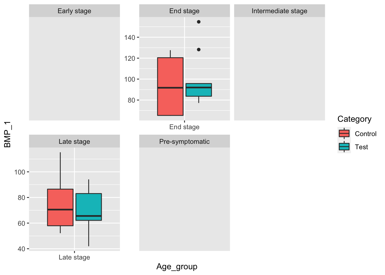 Because much of the BMP_1 data is missing, the only disease stage groups are Late and End stage. We see that the mean in the test group is not larger than the control group. Let’s also try grouping by Sex to see if there is any difference between the mean BMP_2 and BMP_1 level.
# ungrouped ggplot for each output variable (BMP_1,_BMP_2)
ggplot(data, aes(x=Sex, y=BMP_2, fill=Category)) +
    geom_boxplot() +
    facet_wrap(~Sex, scale="free")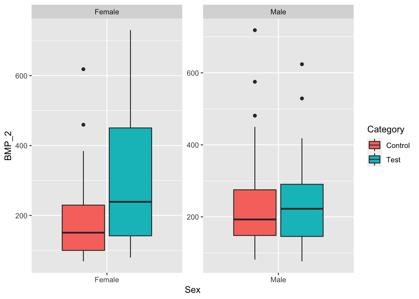
ggplot(data, aes(x=Sex, y=BMP_1, fill=Category)) +
geom_boxplot() +
facet_wrap(~Sex, scale="free")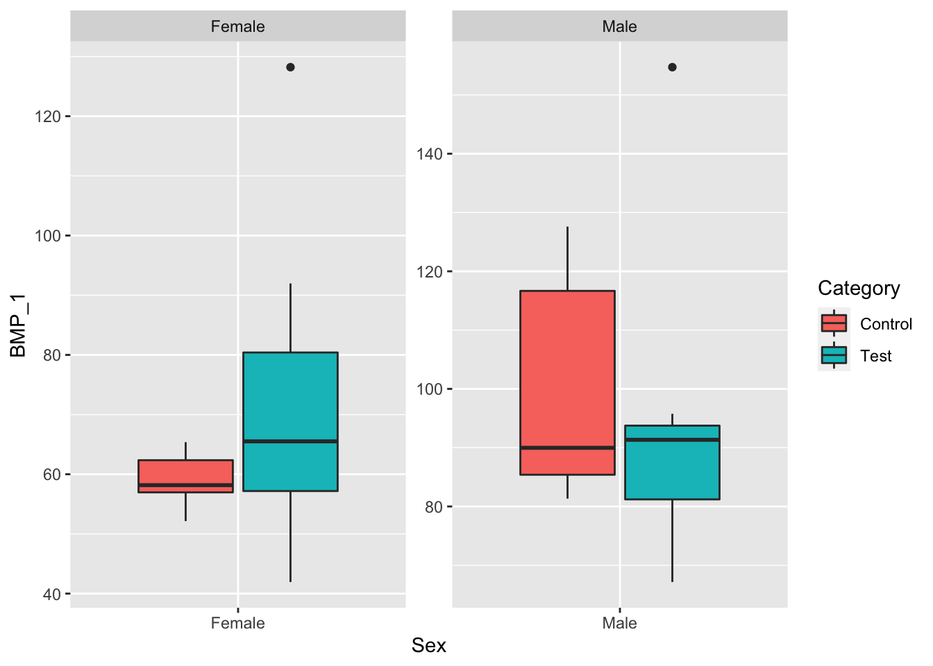 When grouping by Sex only, we see that both test groups have higher mean BMP_1 and BMP_2 levels than their respective control groups.
We can also do filtered box plots for each group given a particular sex.
For Female Mice
# Box plot of BMP_2 for females grouped by disease stage.
female_data <- data[data$Sex == "Female",]
ggplot(female_data, aes(x=Age_group, y=BMP_2, fill=Category)) +
geom_boxplot() +
facet_wrap(~Age_group, scale="free") 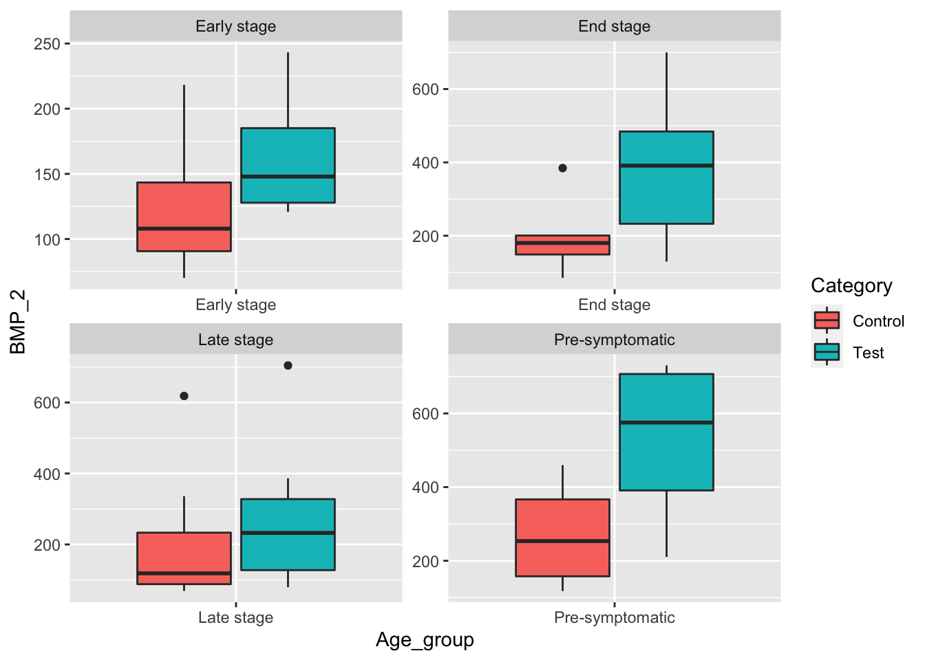 When controlling for Female mice we see that difference between End Stage levels of BMP_1 may be statistically significant.
# Box plot of BMP_1 for females grouped by disease stage.
female_data <- data[data$Sex == "Female",]
ggplot(female_data, aes(x=Age_group, y=BMP_1, fill=Category)) +
geom_boxplot() +
facet_wrap(~Age_group, scale="free")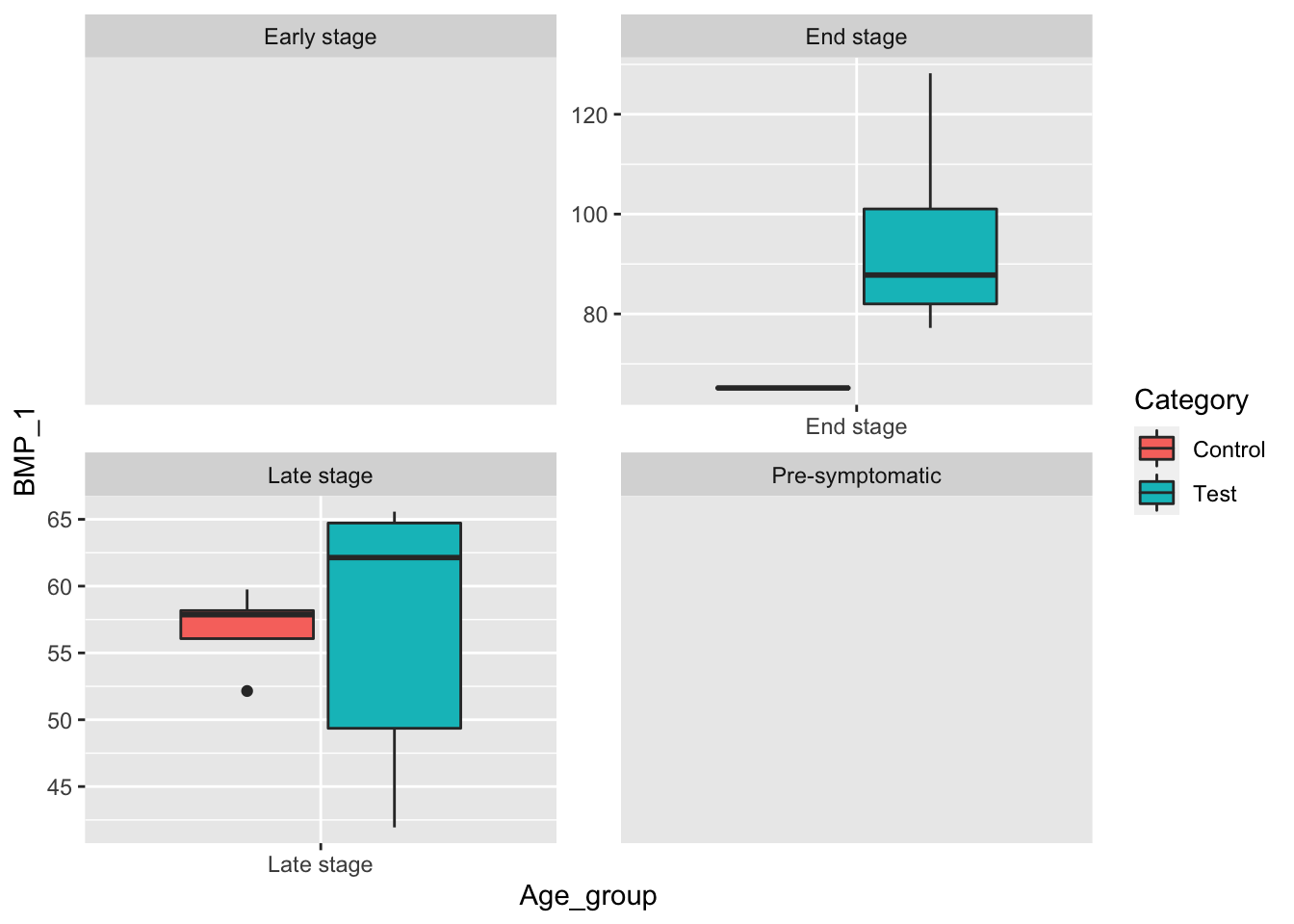 When controlling for female mice, we see that there is a strong case that there is a statistically significant difference in the mean BMP_2 level for the four disease stages given.
For Male Mice
# This is for BMP_1
male_data <- data[data$Sex == "Male",]
ggplot(male_data, aes(x=Age_group, y=BMP_1, fill=Category)) +
geom_boxplot() +
facet_wrap(~Age_group, scale="free")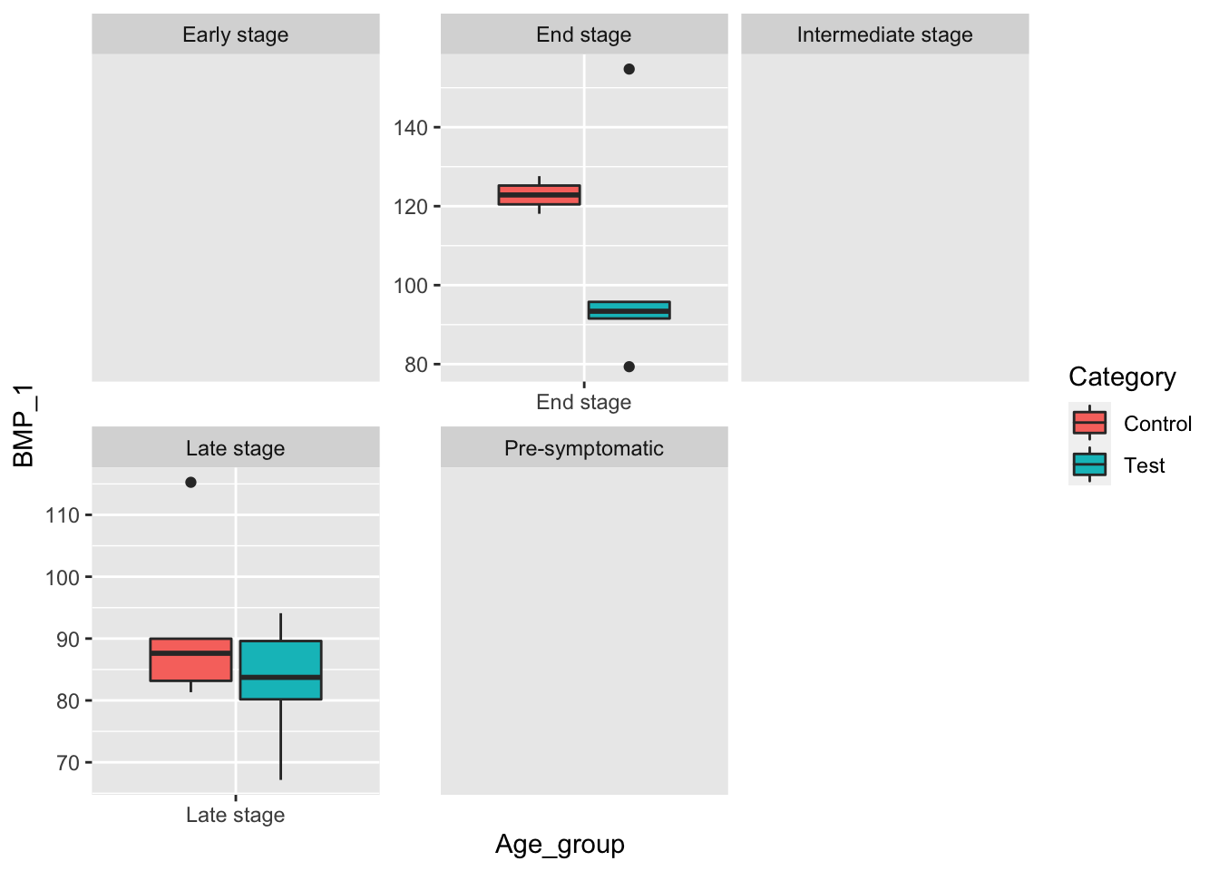 When controlling for male mice we do not see promising data as both control groups have higher mean BMP_1 levels than their test counterparts.
# This is for BMP_2
male_data <- data[data$Sex == "Male",]
ggplot(male_data, aes(x=Age_group, y=BMP_2, fill=Category)) +
geom_boxplot() +
facet_wrap(~Age_group, scale="free")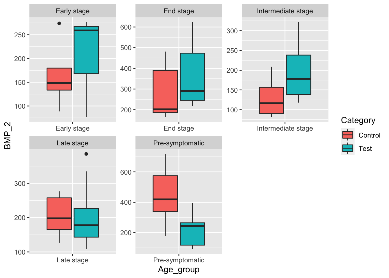 When controlling for male mice, we see some promising results with the mean BMP_2 level being higher in the test groups, when compared to their respective control groups for the disease stages Early, End, and Intermediate Stages.
While these box-whisker plots have mixed results, we will do a Three-Way ANOVA to determine whether the means of each sub-population are equivalent.
# Three-Way ANOVA
# Source: https://stats.oarc.ucla.edu/stata/faq/how-can-i-understand-a-three-way-interaction-in-anova/
# These are great guys ^^^
res.aov2 <- aov(BMP_2 ~ Age_group * Sex * Category, data = data)
#print(summary(res.aov2)[1])
pander(summary(res.aov2),caption="Three-way ANOVA of factors Test/Control, Disease Stage, Sex on BMP_2 levels")| Df | Sum Sq | Mean Sq | F value | Pr(>F) | |
|---|---|---|---|---|---|
| Age_group | 4 | 483777 | 120944 | 5.684 | 0.0004249 |
| Sex | 1 | 5743 | 5743 | 0.2699 | 0.6048 |
| Category | 1 | 52828 | 52828 | 2.483 | 0.1189 |
| Age_group:Sex | 3 | 50050 | 16683 | 0.7841 | 0.5061 |
| Age_group:Category | 4 | 78305 | 19576 | 0.92 | 0.4563 |
| Sex:Category | 1 | 125918 | 125918 | 5.918 | 0.01711 |
| Age_group:Sex:Category | 3 | 173782 | 57927 | 2.722 | 0.04944 |
| Residuals | 84 | 1787347 | 21278 | NA | NA |
The results of the F-test following the ANOVA, we see that the Age Group is a significant factor \(p=0.000426< 0.001\), while neither Sex nor Category are significant factors. However there is a strong interaction effect between Sex and Category, and a small interaction effect between Sex, Age_group and Category. Lets do more ANOVA’s to understand these effects. We will first group by Age_group and run ANOVAs to understand the interaction effect of Sex*Category.
# iterate through the age groups and conduct a 2-way ANOVA for each group
# where the factors are Test/Control and Male/Female, and the output variable is BMP_2 level
for (group in unique(data$Age_group)){
  temp_data <- data[data$Age_group == group,]
  tryCatch({
  temp_anova <- aov(BMP_2 ~ Category*Sex, data=temp_data)
  pander(summary(temp_anova), caption=group)
  }, error=function(e){})
}| Df | Sum Sq | Mean Sq | F value | Pr(>F) | |
|---|---|---|---|---|---|
| Category | 1 | 8701 | 8701 | 0.2792 | 0.6045 |
| Sex | 1 | 33359 | 33359 | 1.071 | 0.3162 |
| Category:Sex | 1 | 277338 | 277338 | 8.9 | 0.00878 |
| Residuals | 16 | 498577 | 31161 | NA | NA |
| Df | Sum Sq | Mean Sq | F value | Pr(>F) | |
|---|---|---|---|---|---|
| Category | 1 | 4926 | 4926 | 0.8394 | 0.3792 |
| Sex | 1 | 5644 | 5644 | 0.9616 | 0.3479 |
| Category:Sex | 1 | 0.1904 | 0.1904 | 3.244e-05 | 0.9956 |
| Residuals | 11 | 64556 | 5869 | NA | NA |
| Df | Sum Sq | Mean Sq | F value | Pr(>F) | |
|---|---|---|---|---|---|
| Category | 1 | 11155 | 11155 | 0.5213 | 0.4757 |
| Sex | 1 | 6329 | 6329 | 0.2958 | 0.5904 |
| Category:Sex | 1 | 8249 | 8249 | 0.3855 | 0.5392 |
| Residuals | 31 | 663361 | 21399 | NA | NA |
| Df | Sum Sq | Mean Sq | F value | Pr(>F) | |
|---|---|---|---|---|---|
| Category | 1 | 103028 | 103028 | 3.916 | 0.06178 |
| Sex | 1 | 4496 | 4496 | 0.1709 | 0.6837 |
| Category:Sex | 1 | 14113 | 14113 | 0.5364 | 0.4724 |
| Residuals | 20 | 526247 | 26312 | NA | NA |
At this stage we run a Tukey Honest Significant Difference test to compare the four groups and determine which groups are different.
# iterate through the age groups and conduct a 2-way ANOVA for each group
# where the factors are Test/Control and Male/Female, and the output variable is BMP_1 level
for (group in unique(data$Age_group)){
  temp_data <- data[data$Age_group == group,]
  tryCatch({
  temp_anova <- aov(BMP_2 ~ Category*Sex, data=temp_data)
  temp_tukey <- TukeyHSD(temp_anova, conf.level=.95)
  pander(temp_tukey,caption=group)
  }, error=function(e){})
  }
## Warning in pander.default(temp_tukey, caption = group): No pander.method for
## "TukeyHSD", reverting to default.No pander.method for "multicomp", reverting to
## default.Category:
diff lwr upr p adj Test-Control -41.93 -210.1 126.3 0.6045 Sex:
diff lwr upr p adj Male-Female -83.08 -253.9 87.72 0.3178 Category:Sex:
diff lwr upr p adj Test:Female-Control:Female 251.6 -105.5 608.8 0.2232 Control:Male-Control:Female 174.5 -164.3 513.3 0.4751 Test:Male-Control:Female -57.36 -373.9 259.2 0.9535 Control:Male-Test:Female -77.16 -416 261.6 0.9134 Test:Male-Test:Female -309 -625.6 7.551 0.05696 Test:Male-Control:Male -231.8 -527.6 63.88 0.1539
## Warning in pander.default(temp_tukey, caption = group): No pander.method for
## "TukeyHSD", reverting to default.No pander.method for "multicomp", reverting to
## default.Category:
diff lwr upr p adj Test-Control 36.33 -50.94 123.6 0.3792 Sex:
diff lwr upr p adj Male-Female 38.78 -48.48 126 0.349 Category:Sex:
diff lwr upr p adj Test:Female-Control:Female 38.9 -124.1 201.9 0.8879 Control:Male-Control:Female 38.77 -124.3 201.8 0.8888 Test:Male-Control:Female 78.12 -97.96 254.2 0.5613 Control:Male-Test:Female -0.13 -163.2 162.9 1 Test:Male-Test:Female 39.22 -136.9 215.3 0.9061 Test:Male-Control:Male 39.35 -136.7 215.4 0.9053
## Warning in pander.default(temp_tukey, caption = group): No pander.method for
## "TukeyHSD", reverting to default.No pander.method for "multicomp", reverting to
## default.Category:
diff lwr upr p adj Test-Control 35.72 -65.18 136.6 0.4757 Sex:
diff lwr upr p adj Male-Female -26.98 -128.2 74.25 0.5906 Category:Sex:
diff lwr upr p adj Test:Female-Control:Female 63.25 -119.2 245.7 0.7831 Control:Male-Control:Female 4.577 -188.3 197.5 0.9999 Test:Male-Control:Female 6.153 -186.8 199.1 0.9998 Control:Male-Test:Female -58.67 -247 129.7 0.8323 Test:Male-Test:Female -57.1 -245.4 131.2 0.8432 Test:Male-Control:Male 1.576 -196.9 200.1 1
## Warning in pander.default(temp_tukey, caption = group): No pander.method for
## "TukeyHSD", reverting to default.No pander.method for "multicomp", reverting to
## default.Category:
diff lwr upr p adj Test-Control 131.5 -7.123 270.1 0.06178 Sex:
diff lwr upr p adj Male-Female 27.47 -111.2 166.1 0.6837 Category:Sex:
diff lwr upr p adj Test:Female-Control:Female 184.7 -90.26 459.6 0.2678 Control:Male-Control:Female 80.44 -194.5 355.4 0.8448 Test:Male-Control:Female 167.4 -98.43 433.3 0.3196 Control:Male-Test:Female -104.2 -366.3 157.9 0.686 Test:Male-Test:Female -17.25 -269.8 235.3 0.9974 Test:Male-Control:Male 86.97 -165.6 339.6 0.7711
While this may seem like a lot of information Lets make a table for the adjusted p-value for the groups we are actually interested in comparing.
Table 2
| Disease Stage | Sex | Adjusted p value |
|---|---|---|
| Pre-Symptomatic | Male | 0.1610516 |
| Pre-Symptomatic | Female | 0.2267875 |
| Early Stage | Male | 0.9211629 |
| Early Stage | Female | 0.8947598 |
| Intermediate Stage | Male | |
| Late Stage | Male | 0.9999997 |
| Late Stage | Female | 0.7663138 |
| End Stage | Male | 0.7643094 |
| End Stage | Female | 0.2709241 |
From Table 2 we see that difference in means between the test/control groups were not significantly different. Proceeding from here, it may make sense to develop a linear model for how the BMP_2 and BMP_1 increase as the mouse gets to later stages in the disease.
Repeating this process for BMP_1 Lets first take the Three-way ANOVA
res.aov2 <- aov(BMP_1 ~ Age_group * Sex * Category, data = data)
pander(summary(res.aov2),caption="Three-way ANOVA where the output variable is BMP_1 level, and the factors are Disease stage, Sex, Test/Control")| Df | Sum Sq | Mean Sq | F value | Pr(>F) | |
|---|---|---|---|---|---|
| Age_group | 1 | 5874 | 5874 | 23.69 | 3.989e-05 |
| Sex | 1 | 6894 | 6894 | 27.8 | 1.316e-05 |
| Category | 1 | 16.91 | 16.91 | 0.0682 | 0.7959 |
| Age_group:Sex | 1 | 90.61 | 90.61 | 0.3654 | 0.5504 |
| Age_group:Category | 1 | 125.1 | 125.1 | 0.5044 | 0.4835 |
| Sex:Category | 1 | 1014 | 1014 | 4.091 | 0.05276 |
| Age_group:Sex:Category | 1 | 804.2 | 804.2 | 3.243 | 0.0825 |
| Residuals | 28 | 6943 | 248 | NA | NA |
Here we see that Category is again not a significant factor, but factors for Age_group and Sex are significant. There is a small interaction effect between Sex and Category that may be worth investigating. We again take an Two-way ANOVAs for each Age_group.
# iterate through the age groups and conduct a 2-way ANOVA for each group
# where the factors are Test/Control and Male/Female, and the output variable is BMP_1 level
for (group in unique(data$Age_group)){
temp_data <- data[data$Age_group == group,]
tryCatch({
temp_anova <- aov(BMP_1 ~ Category*Sex, data=temp_data)
pander(summary(temp_anova), caption=group)
}, error=function(e){})
}| Df | Sum Sq | Mean Sq | F value | Pr(>F) | |
|---|---|---|---|---|---|
| Category | 1 | 148.8 | 148.8 | 1.546 | 0.2289 |
| Sex | 1 | 5157 | 5157 | 53.59 | 6.106e-07 |
| Category:Sex | 1 | 96.89 | 96.89 | 1.007 | 0.3283 |
| Residuals | 19 | 1829 | 96.24 | NA | NA |
| Df | Sum Sq | Mean Sq | F value | Pr(>F) | |
|---|---|---|---|---|---|
| Category | 1 | 84.55 | 84.55 | 0.1488 | 0.7087 |
| Sex | 1 | 1736 | 1736 | 3.055 | 0.1144 |
| Category:Sex | 1 | 1722 | 1722 | 3.03 | 0.1157 |
| Residuals | 9 | 5114 | 568.3 | NA | NA |
It should not be much of a surprise that the results of the Two-way ANOVA show that the difference between the groups is largely due to sex. We will do a Tukey HSD test again to illustrate which groups are different.
# source: https://www.r-bloggers.com/2021/08/how-to-perform-tukey-hsd-test-in-r/
for (group in unique(data$Age_group)){
temp_data <- data[data$Age_group == group,]
tryCatch({
temp_anova <- aov(BMP_1 ~ Category*Sex, data=temp_data)
temp_tukey <- TukeyHSD(temp_anova, conf.level=.95)
pander(temp_tukey,caption=group)
}, error=function(e){})
}## Warning in pander.default(temp_tukey, caption = group): No pander.method for
## "TukeyHSD", reverting to default.No pander.method for "multicomp", reverting to
## default.Category:
diff lwr upr p adj Test-Control -5.13 -13.77 3.507 0.2289 Sex:
diff lwr upr p adj Male-Female 29.95 21.38 38.53 6.17e-07 Category:Sex:
diff lwr upr p adj Test:Female-Control:Female 0.03029 -16.12 16.18 1 Control:Male-Control:Female 34.67 17.23 52.12 0.0001184 Test:Male-Control:Female 26.41 9.708 43.12 0.00145 Control:Male-Test:Female 34.64 18.49 50.79 4.625e-05 Test:Male-Test:Female 26.38 11.03 41.73 0.0006142 Test:Male-Control:Male -8.261 -24.96 8.442 0.52
## Warning in pander.default(temp_tukey, caption = group): No pander.method for
## "TukeyHSD", reverting to default.No pander.method for "multicomp", reverting to
## default.Category:
diff lwr upr p adj Test-Control 5.526 -26.88 37.93 0.7087 Sex:
diff lwr upr p adj Male-Female 23.15 -6.851 53.15 0.1148 Category:Sex:
diff lwr upr p adj Test:Female-Control:Female 30.08 -34.37 94.53 0.4986 Control:Male-Control:Female 57.67 -16.75 132.1 0.1424 Test:Male-Control:Female 37.79 -24.48 100 0.2952 Control:Male-Test:Female 27.59 -36.86 92.04 0.5648 Test:Male-Test:Female 7.705 -42.22 57.63 0.9612 Test:Male-Control:Male -19.89 -82.15 42.38 0.7549
Table 3
| Disease Stage | Sex | Adjusted p value |
|---|---|---|
| Late Stage | Male | 0.3621039 |
| Late Stage | Female | 0.9881989 |
| End Stage | Male | 0.7601283 |
| End Stage | Female | 0.4879153 |
From Table 3 we see that the groups of interest are not responsible for the difference between the means of the four groups.
Multiple Regression
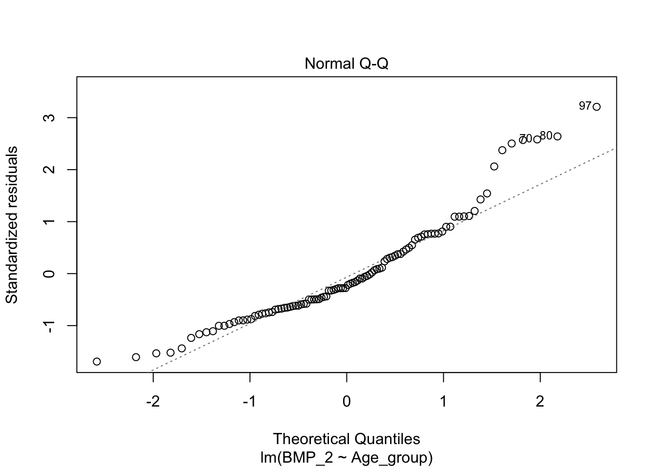
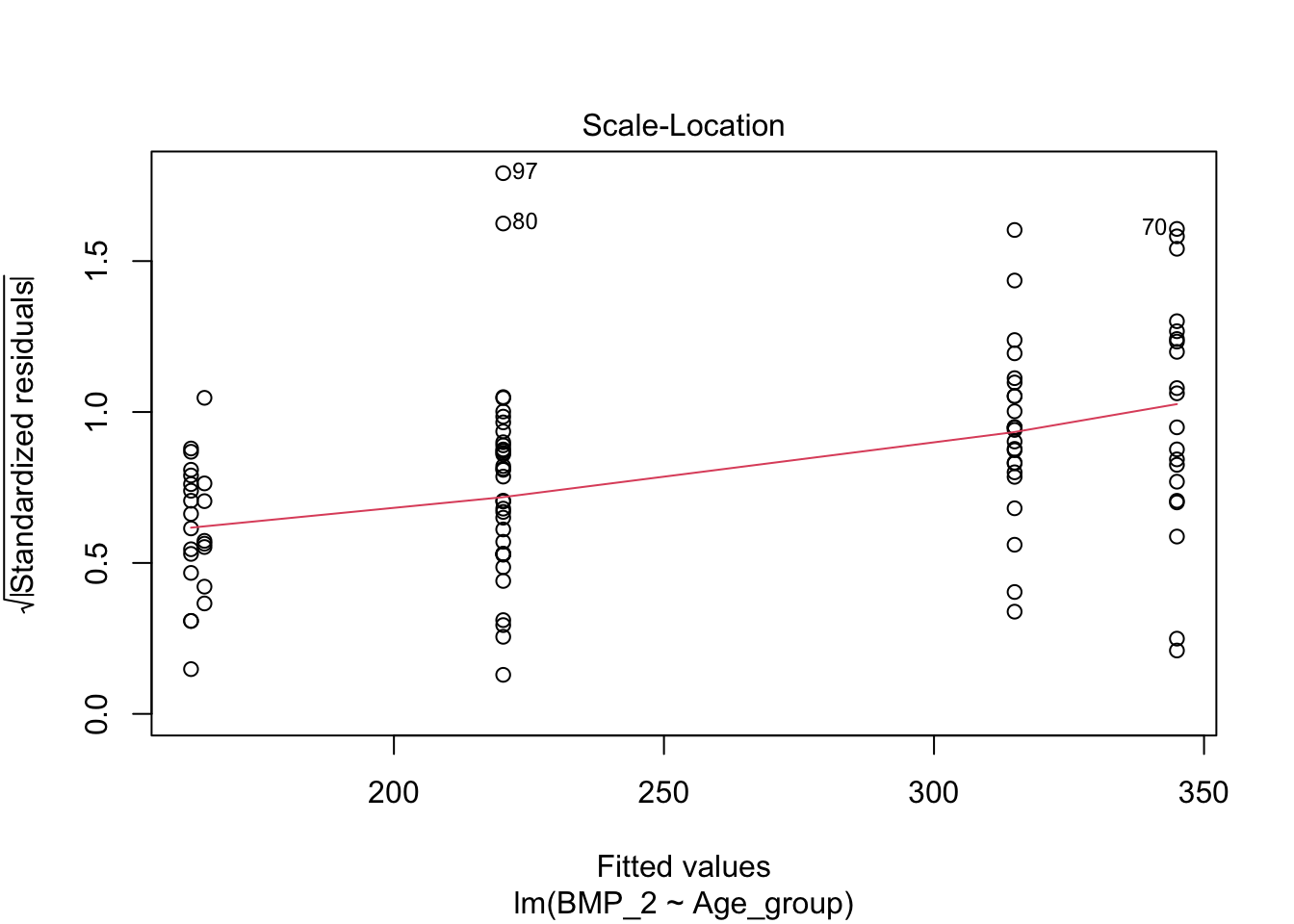
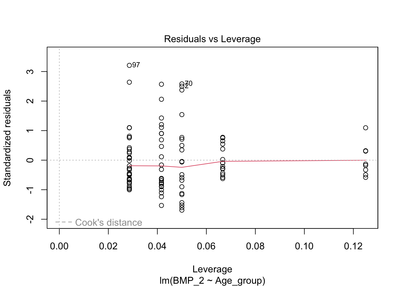
A linear model can developed to associate the disease stage with the level of BMP_2 and BMP_1. This is resolved in the ANOVA, but not explicitly investigated.
linearmodel <- lm(BMP_2 ~ Age_group, data = data)
plot(linearmodel)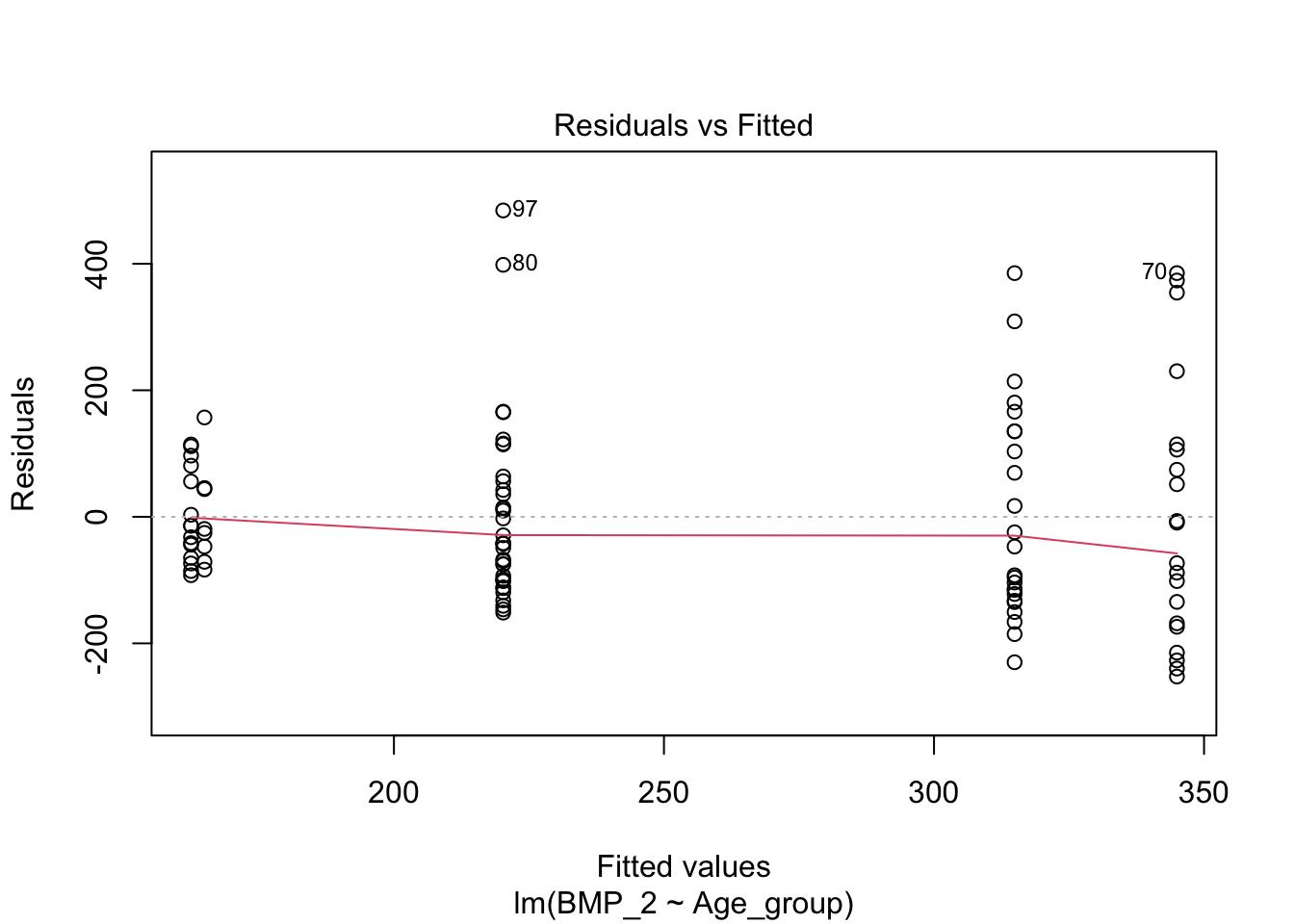
pander(summary(linearmodel))| Estimate | Std. Error | t value | Pr(>|t|) | |
|---|---|---|---|---|
| (Intercept) | 162.4 | 39.53 | 4.109 | 8.319e-05 |
| Age_groupEnd stage | 152.5 | 50.4 | 3.026 | 0.003173 |
| Age_groupIntermediate stage | 2.491 | 67.03 | 0.03716 | 0.9704 |
| Age_groupLate stage | 57.81 | 47.25 | 1.223 | 0.2241 |
| Age_groupPre-symptomatic | 182.5 | 52.3 | 3.491 | 0.0007269 |
| Observations | Residual Std. Error | \(R^2\) | Adjusted \(R^2\) |
|---|---|---|---|
| 102 | 153.1 | 0.1754 | 0.1414 |
T-tests if you need them
T-tests are included but not recommended because of significant increase in the Family Wise error rate. Meaning you are more likely to have a false positive in your results.
By Sex
# t tests by sex
pander(t.test (BMP_2 ~ Category , var.equal=TRUE, alternative="less", data = subset(data, Sex == "Male")))
##
## --------------------------------------------------------------------------------
## Test statistic df P value Alternative hypothesis mean in group Control
## ---------------- ---- --------- ------------------------ -----------------------
## 0.09206 54 0.5365 less 249.1
## --------------------------------------------------------------------------------
##
## Table: Two Sample t-test: `BMP_2` by `Category` (continued below)
##
##
## --------------------
## mean in group Test
## --------------------
## 245.6
## --------------------t.test (BMP_2 ~ Category , var.equal=TRUE, alternative="less", data = subset(data, Sex == "Female"))##
## Two Sample t-test
##
## data: BMP_2 by Category
## t = -2.242, df = 44, p-value = 0.01503
## alternative hypothesis: true difference in means between group Control and group Test is less than 0
## 95 percent confidence interval:
## -Inf -30.31352
## sample estimates:
## mean in group Control mean in group Test
## 199.3309 320.3100t.test (BMP_1 ~ Category , var.equal=TRUE, alternative="less", data = subset(data, Sex == "Male"))##
## Two Sample t-test
##
## data: BMP_1 by Category
## t = 0.80213, df = 16, p-value = 0.7829
## alternative hypothesis: true difference in means between group Control and group Test is less than 0
## 95 percent confidence interval:
## -Inf 26.20367
## sample estimates:
## mean in group Control mean in group Test
## 100.43500 92.18595t.test (BMP_1 ~ Category , var.equal=TRUE, alternative="less", data = subset(data, Sex == "Female"))##
## Two Sample t-test
##
## data: BMP_1 by Category
## t = -1.2369, df = 16, p-value = 0.117
## alternative hypothesis: true difference in means between group Control and group Test is less than 0
## 95 percent confidence interval:
## -Inf 4.777702
## sample estimates:
## mean in group Control mean in group Test
## 59.19129 70.80095By Group
ttest_table <- function(data,bmp1or2){
  dstage <-degfree <-tstat <- pval <- c()
  for (stage in unique(data$Age_group)){
    tryCatch({
      if (bmp1or2){
        ttest <- t.test(BMP_1 ~ Category , var.equal=TRUE, alternative="less", data = subset(data, Age_group == stage))
      }else{
        ttest <- t.test(BMP_2 ~ Category , var.equal=TRUE, alternative="less", data = subset(data, Age_group == stage))
      }
      degfree <- c(degfree,ttest$parameter)
      tstat <- c(tstat,ttest$statistic)
      pval <- c(pval,ttest$p.value)
      dstage <- c(dstage,stage)
      }, error=function(e){})
  }
  return(data.frame(dstage,degfree,tstat,pval))
  }
kable(ttest_table(data,bmp1or2=TRUE),caption="bmp1 t-test results") | dstage | degfree | tstat | pval |
|---|---|---|---|
| Late stage | 21 | 0.6641166 | 0.7430790 |
| End stage | 11 | -0.3293894 | 0.3740241 |
kable(ttest_table(data,bmp1or2=FALSE),caption="bmp2 t-test results") | dstage | degfree | tstat | pval |
|---|---|---|---|
| Pre-symptomatic | 18 | 0.4399299 | 0.6673876 |
| Early stage | 13 | -0.9551325 | 0.1784677 |
| Intermediate stage | 6 | -1.2689540 | 0.1257301 |
| Late stage | 33 | -0.7368671 | 0.2332050 |
| End stage | 22 | -2.0396158 | 0.0267883 |
By Group Given that the mouse is Female
female_data <- data[data$Sex == "Female",]
kable(ttest_table(female_data,bmp1or2=TRUE),caption="bmp1 t-test results") | dstage | degfree | tstat | pval |
|---|---|---|---|
| Late stage | 10 | -0.0066006 | 0.4974317 |
| End stage | 4 | -1.7594741 | 0.0766554 |
kable(ttest_table(female_data,bmp1or2=FALSE),caption="bmp2 t-test results") | dstage | degfree | tstat | pval |
|---|---|---|---|
| Pre-symptomatic | 6 | -1.7437019 | 0.0659169 |
| Early stage | 6 | -0.9130563 | 0.1982090 |
| Late stage | 17 | -0.7515993 | 0.2312857 |
| End stage | 9 | -1.7655825 | 0.0556395 |
By Group Given that the mouse is Male
male_data <- data[data$Sex == "Male",]
kable(ttest_table(male_data,bmp1or2=TRUE),caption="bmp1 t-test results") | dstage | degfree | tstat | pval |
|---|---|---|---|
| Late stage | 9 | 1.174397 | 0.8648135 |
| End stage | 5 | 0.891278 | 0.7931956 |
kable(ttest_table(male_data,bmp1or2=FALSE),caption="bmp2 t-test results") | dstage | degfree | tstat | pval |
|---|---|---|---|
| Pre-symptomatic | 10 | 2.5109369 | 0.9845685 |
| Early stage | 5 | -0.5570914 | 0.3007404 |
| Intermediate stage | 6 | -1.2689540 | 0.1257301 |
| Late stage | 14 | -0.0386572 | 0.4848548 |
| End stage | 11 | -1.0212576 | 0.1645340 |
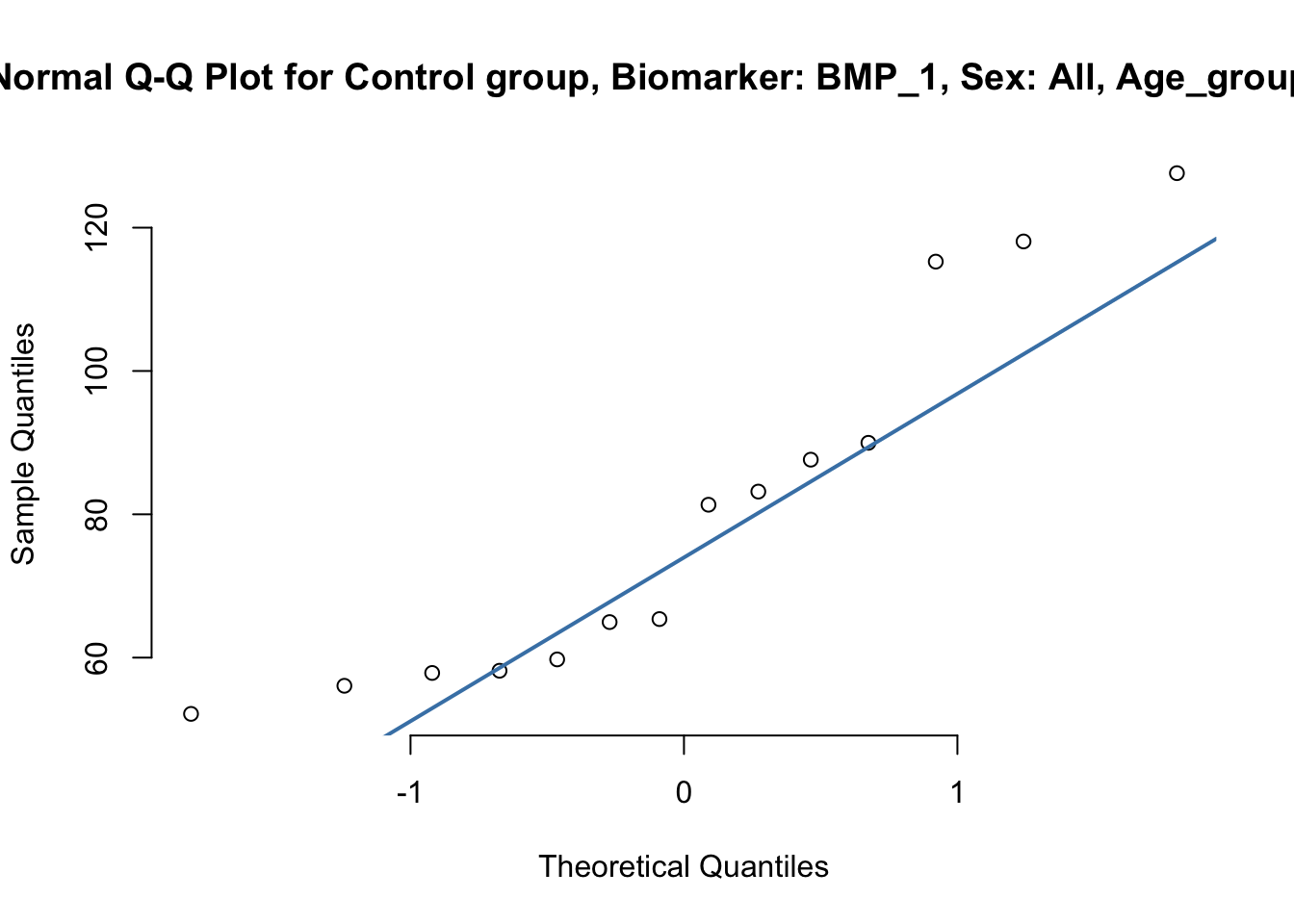
Appendix
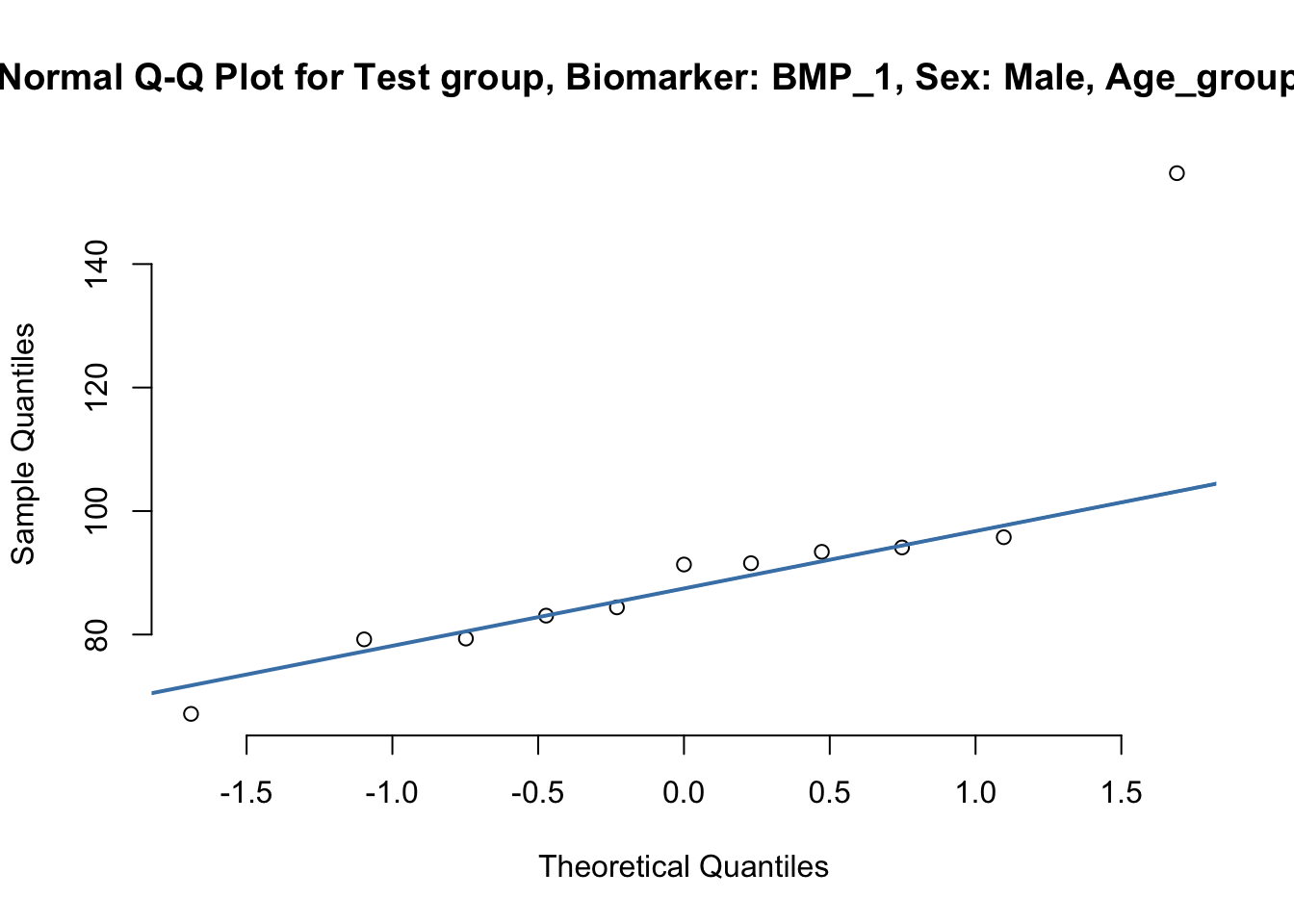
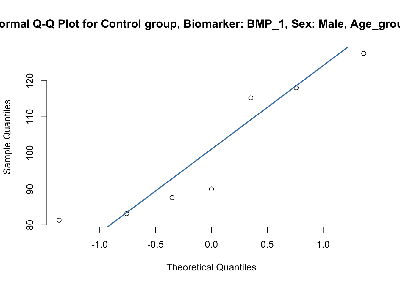
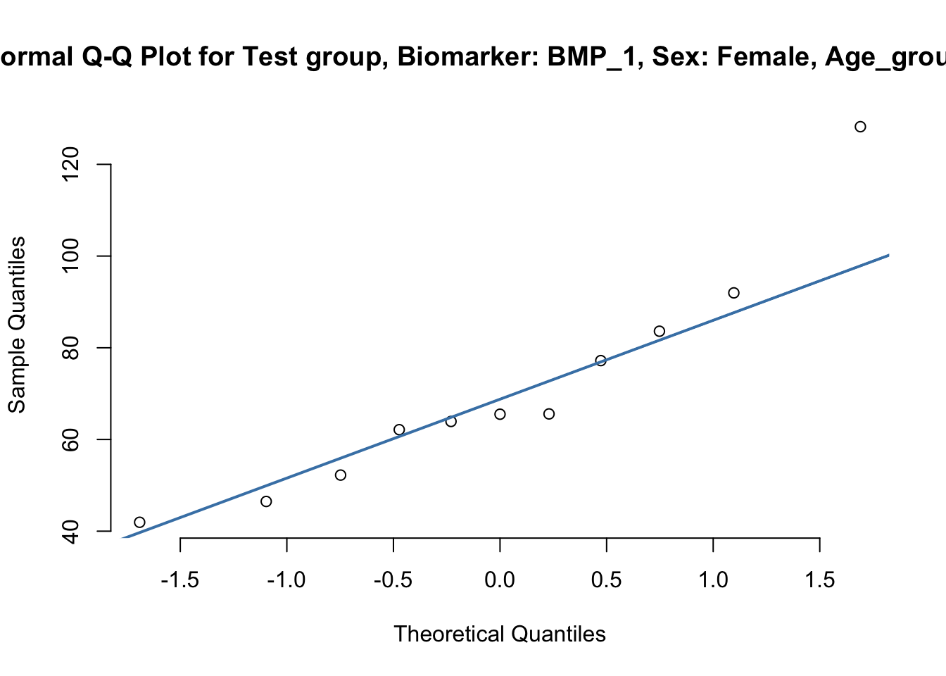
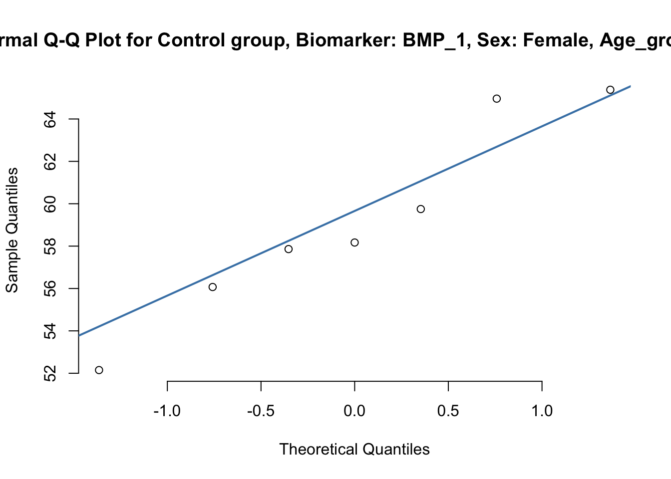
This section contains the QQ plots and tests of normality for each variable.
# The kinds of QQ plots for each ANOVA are

# creating Q-Q plot for each group.
QQplotter_BMP_1 <- function(dataset, s, ag){
  test <-  dataset[dataset$Category == "Test",]
  control <- dataset[dataset$Category == "Control", ]
  qqnorm(test$BMP_1, pch=1, frame=FALSE, main=sprintf("Normal Q-Q Plot for Test group, Biomarker: BMP_1, Sex: %s, Age_group: %s", s, ag))
  qqline(test$BMP_1, col = "steelblue", lwd = 2)
  qqnorm(control$BMP_1,pch=1, frame=FALSE, main=sprintf("Normal Q-Q Plot for Control group, Biomarker: BMP_1, Sex: %s, Age_group: %s", s, ag))
  qqline(control$BMP_1, col = "steelblue", lwd = 2)
}

# Total
QQplotter_BMP_1(data, s="All", ag="All")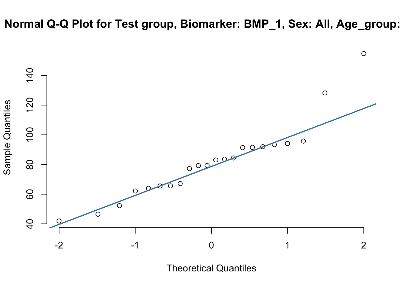
# By Sex
for (sex in unique(data$Sex)){
  temp_data <-  data[data$Sex == sex,]
  QQplotter_BMP_1(temp_data,s=sex, ag="All")
}
# By Group
for (group in unique(data$Age_group)){
  tryCatch({
    temp_data <-  data[data$Sex == group,]
  QQplotter_BMP_1(temp_data,s="All", ag=group)
  }, error=function(e){})
}
# By Group Given Sex is Male
male_data <- data[data$Sex == "Male",]
for (group in unique(male_data$Age_group)){
  tryCatch({
    temp_data <-  male_data[male_data$Sex == group,]
  QQplotter_BMP_1(temp_data,s="All", ag=group)
  }, error=function(e){})
}
# By Group Given Sex is Female
male_data <- data[data$Sex == "Female",]
for (group in unique(male_data$Age_group)){
  tryCatch({
    temp_data <-  male_data[male_data$Sex == group,]
  QQplotter_BMP_1(temp_data,s="All", ag=group)
  }, error=function(e){})
}