Exploratory Data Analysis for Undisclosed Client
This project focuses on determining if there is a statistically significant difference in biomarker protein levels (BMP) in patients with a genetic disease. There are too few participants to take advantage of the robustness to non-normality for the t-test. However we will first assess normality using Q-Q plots, and the Shapiro-Wilks test. We will then test the means of each sample to determine whether the difference in the population means are statistically different from 0. From these results we explore possible avenues for alternative tests, further testing, and future study design.
First lets look at the data.
library(dplyr)
library(psych)
library(knitr)
library(pander)
data <- read.csv("dummdata.csv", header=TRUE, stringsAsFactors=TRUE)
test <- subset(data, Category == "Test")
control <- subset(data, Category == "Control")
plot(data)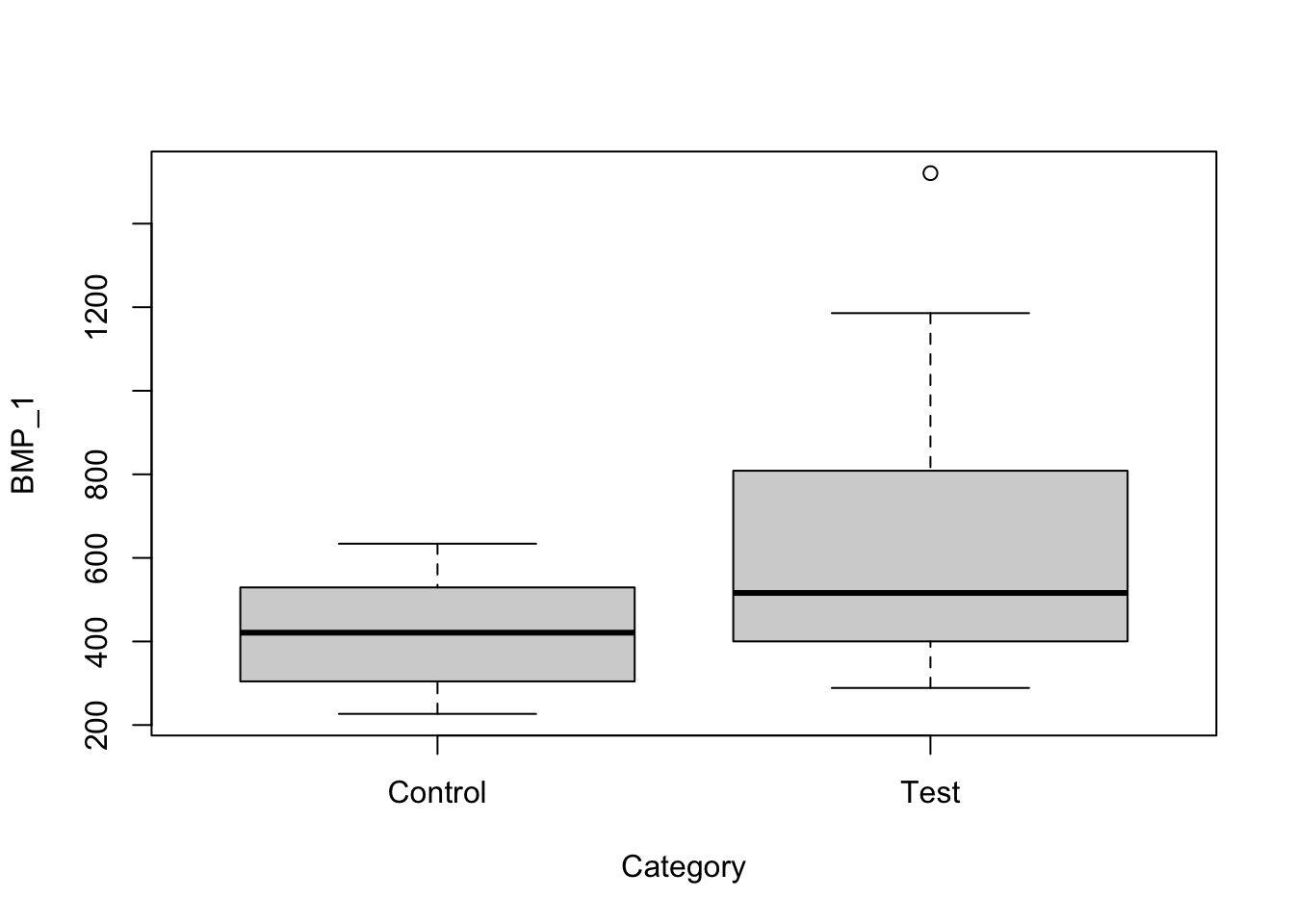
kable(describe(data,skew=FALSE),caption="Basic Statistics on BMP levels")| vars | n | mean | sd | min | max | range | se | |
|---|---|---|---|---|---|---|---|---|
| Category* | 1 | 24 | 1.541667 | 0.5089774 | 1.0000 | 2.000 | 1.000 | 0.1038946 |
| BMP_1 | 2 | 24 | 554.180041 | 310.2578414 | 226.6834 | 1520.845 | 1294.162 | 63.3311167 |
From the data we see that there may be a statistically significant difference between the population means. However, since the sample size is small (n<40) we must first determine using Q-Q plots that the distribution of the sample is approximately normally distributed.
qqnorm(test$BMP_1, pch=1, frame=FALSE, main="Normal Q-Q Plot for Test group")
qqline(test$BMP_1, col = "steelblue", lwd = 2)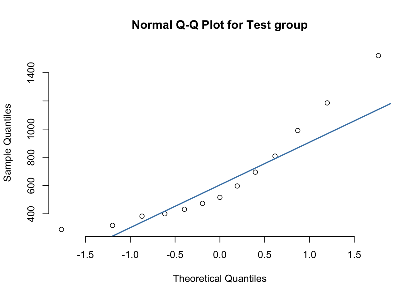
qqnorm(control$BMP_1,pch=1, frame=FALSE, main="Normal Q-Q Plot for Control group")
qqline(control$BMP_1, col = "steelblue", lwd = 2)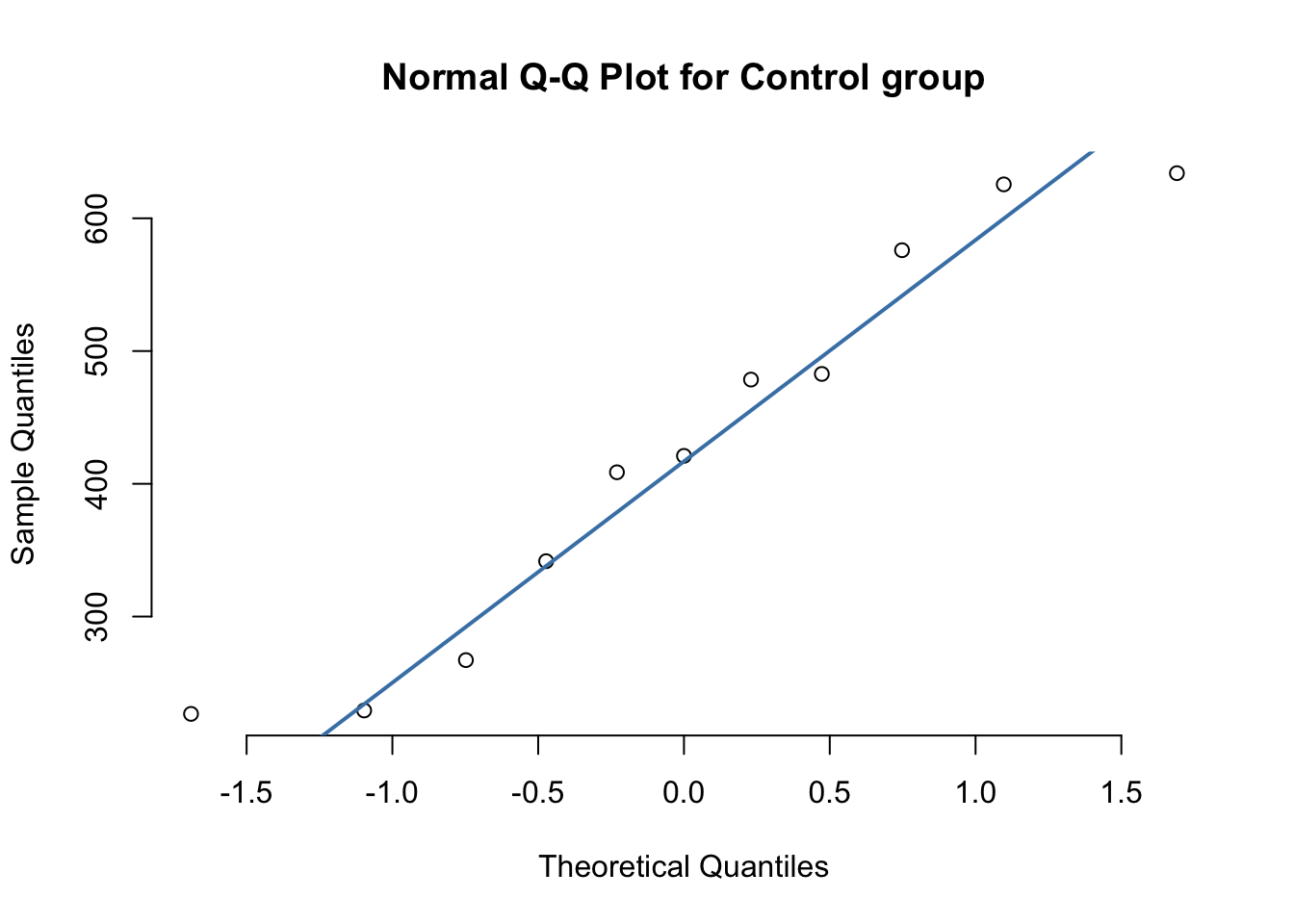
#Test each group for normality
data %>%
  group_by(Category) %>%
  summarise(`W Stat` = shapiro.test(BMP_1)$statistic,
            p.value = shapiro.test(BMP_1)$p.value)
## # A tibble: 2 × 3
## Category `W Stat` p.value
## <fct> <dbl> <dbl>
## 1 Control 0.927 0.383
## 2 Test 0.868 0.0494From the preliminary Q-Q plots we see that each group is sufficiently normally distributed. The Shapiro-Wilks test also confirms this cursory inspection.
We use a t-test to determine if there is a statistically significant difference between sample means. We define our null(\(H_0\)) and alternativ(e(\(H_a\)) hypotheses as \[ H_0: \mu_{test} - \mu_{control} = 0 \] \[ H_a: \mu_{test} - \mu_{control} > 0\].
We assume the population variances are equal for this first test.
# source
# http://www.cookbook-r.com/Statistical_analysis/t-test/
t.test (BMP_1 ~ Category , var.equal=TRUE, alternative="less", data = data)
##
## Two Sample t-test
##
## data: BMP_1 by Category
## t = -1.967, df = 22, p-value = 0.03096
## alternative hypothesis: true difference in means between group Control and group Test is less than 0
## 95 percent confidence interval:
## -Inf -29.94641
## sample estimates:
## mean in group Control mean in group Test
## 426.4854 662.2293At the level of \(\alpha=0.05\), we can reject \(H_0\). Since we have insufficient understanding of the variances of each population, we can also try the t-test assuming variances are different.
t.test (BMP_1 ~ Category , var.equal=FALSE, alternative="less", data = data)##
## Welch Two Sample t-test
##
## data: BMP_1 by Category
## t = -2.0947, df = 16.291, p-value = 0.02609
## alternative hypothesis: true difference in means between group Control and group Test is less than 0
## 95 percent confidence interval:
## -Inf -39.46911
## sample estimates:
## mean in group Control mean in group Test
## 426.4854 662.2293While these results seem promising, further exploration into power analysis and minimum effect size should be researched. If we are expecting small population samples, we may have to employ bootstrap methods to estimate population confidence intervals. Below we comopute a distribution of sample means by resampling from our sample set with replacement. We show a box plot to illustrate the bootstrapped population distribution.
# source:
# https://home.uncg.edu/mat/qms/Resampling%20Methods%20Using%20R.pdf
BMP_1_ctrl <- c(control$BMP_1)
BMP_1_test <- c(test$BMP_1)

get_bootstrap <- function(num_boots, data) {
  # function that will generate a vector of
  # biomarker data from resampling from the biomarker
  # data with replacement.
  #
  # Parameters
  # ----------
  # data : vector of numerics
  #   biomarker data, assumed to be small
  #
  # Returns
  # -------
  # boot.result : vector of numerics
  #   boot strapped biomarker data

  N <- length(data)
  nboots <- num_boots
  boot.result <- numeric(nboots)
  for(i in 1:nboots){
    boot.samp <- sample(data, N, replace=TRUE)
    boot.result[i] <- mean(boot.samp)
  }
  return(boot.result)
}

ctrl_boot <- get_bootstrap(100, BMP_1_ctrl)
test_boot <- get_bootstrap(100, BMP_1_test)

hist(ctrl_boot)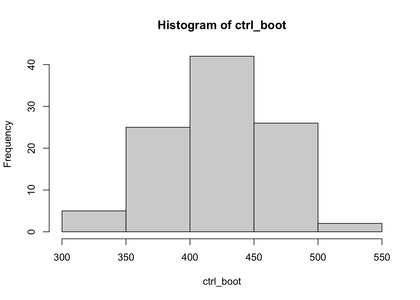
hist(test_boot)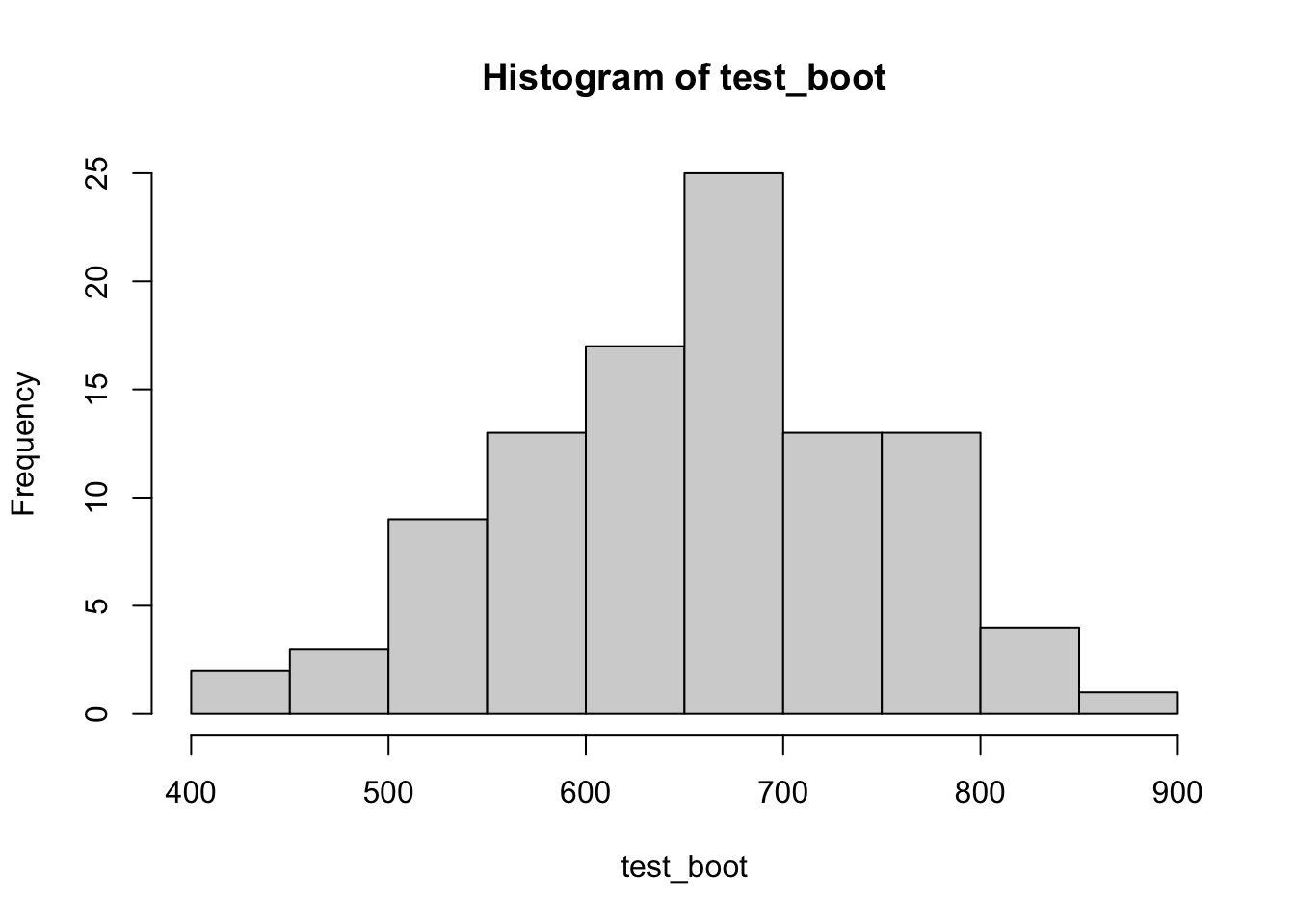
boxplot(ctrl_boot, test_boot)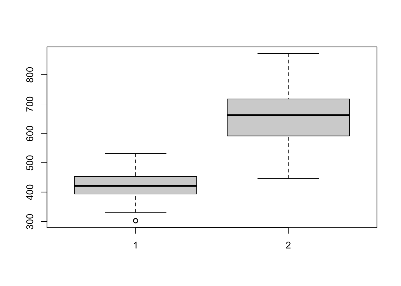
t.test(ctrl_boot, test_boot, var.equal=FALSE)##
## Welch Two Sample t-test
##
## data: ctrl_boot and test_boot
## t = -23.13, df = 140.78, p-value < 2.2e-16
## alternative hypothesis: true difference in means is not equal to 0
## 95 percent confidence interval:
## -253.6993 -213.7463
## sample estimates:
## mean of x mean of y
## 422.8000 656.5228From these results the means boot-strapped population distributions are very much unequal. We can talk more about bootstrapping if it interests you.
Client asked about the Mann-Whitney U test. This test is a non-parametric test that is used when little is known about the distribution from which you are sampling from. Results from this test are inconclusive.
# source:
# https://stat-methods.com/home/mann-whitney-u-r/
#Perform the Mann-Whitney U test
m1<-wilcox.test(BMP_1 ~ Category, data=data, na.rm=TRUE, paired=FALSE, exact=FALSE, conf.int=TRUE)
pander(m1,caption="ManWitney U test on BMP_1")| Test statistic | P value | Alternative hypothesis | difference in location |
|---|---|---|---|
| 45 | 0.132 | two.sided | -153.7 |